As many of you requested I have posted the recording titled "Reporting on a Fault Tree Model" . In this webinar we showed a few of the many features available in the report designer.
One of the most important aspects of your reliability or safety studies is the creation of professional standard reports that will enable you to present the results in a clear and understandable form to colleagues, management, customers and regulatory bodies.
HOW CAN I USE THE REPORT DESIGNER?
The Isograph reliability software products share a common facility to produce reports containing text, graphs or diagrams. Your input data and output results from reliability applications are stored in a database. This information can be examined, filtered, sorted and displayed by the Report Designer. The Report Designer allows you to use reports supplied by Isograph to print or print preview the data. A set of report format appropriate to the product is supplied with each product.
You can also design your own reports, either from an empty report page or by copying one of the supplied reports and using that as the starting point.
Reports may published or exported to PDF and Word formats.
As always please feel free to contact me if you have any questions: jhynek@mttf.info .
Howdy, folks. Jeremy mentioned it was coming a few months back, but now it's finally here! The Isograph Network Availability Prediction (NAP) 2.0 official release happened under our noses a few weeks ago. I wanted to talk about this product and the new updates to it.
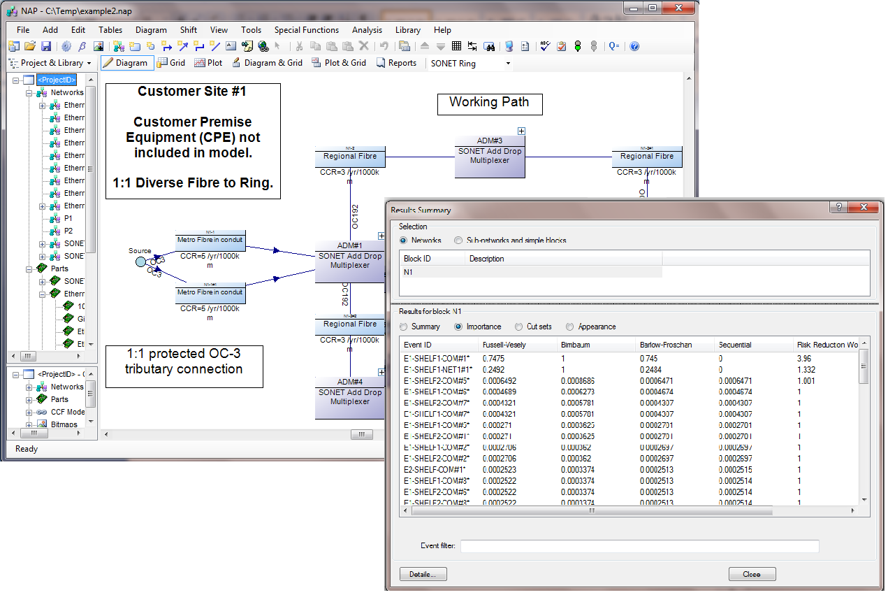
Network Availability Prediction (NAP) 2.0 features an updated user interface, sharing common functionality with the Reliability and Availability Workbench products.
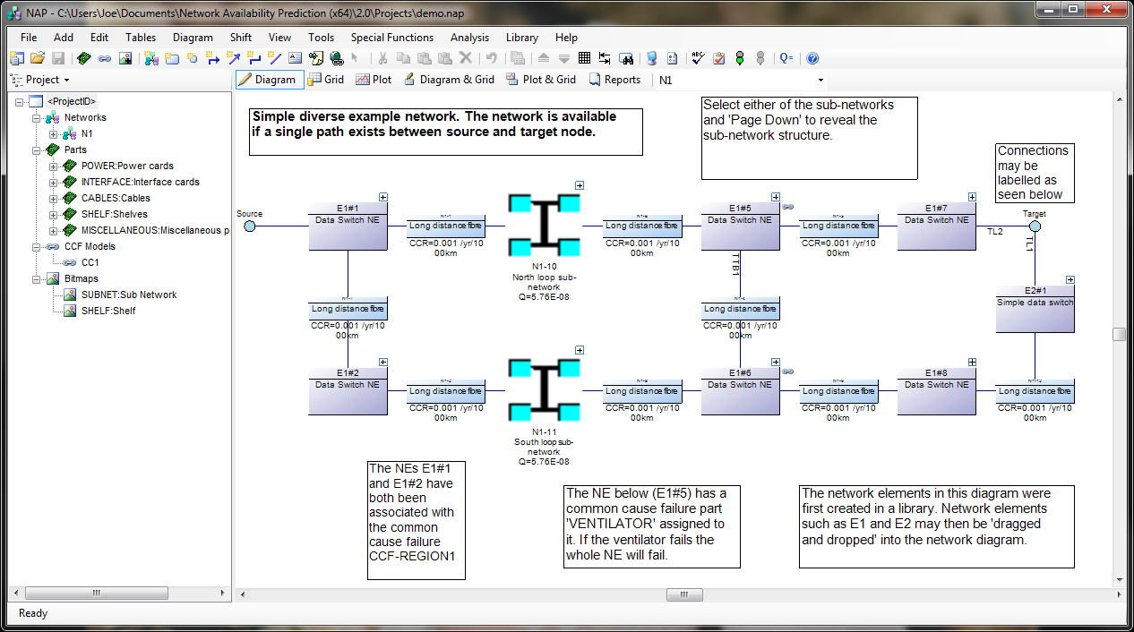
NAP is one of our lesser-used products. It's not as common as Fault Tree or RCMCost, so I'll introduce you to it first, in case you haven't heard of it. NAP is an extension of the analytical RBD methodologies found in Reliability Workbench. It's based on an RBD, but the RBD features have been expanded a great deal in order to allow modeling of telecommunications networks. These Network Block Diagrams (NBDs) differ from RBDs in that they allow for two-way connections and sockets.
In traditional RBDs, a connection only allows for a one-way logical flow, and each block diagram must have a single input and output. This makes the block diagram evaluation simple, but makes it difficult to evaluate complex communications networks. NBDs are an expansion of that. The two-way flow along connections allows more complex systems modeling, and sockets allow each block diagram to have multiples inputs and outputs. When evaluating, NAP will find all valid paths through the system, from the top level source to target nodes. The network diagram must still have a single source-target pair at the highest level; this is how availability is measured. Once it's identified all paths, then it will determine the cut sets that would block all possible paths, much like an RBD.
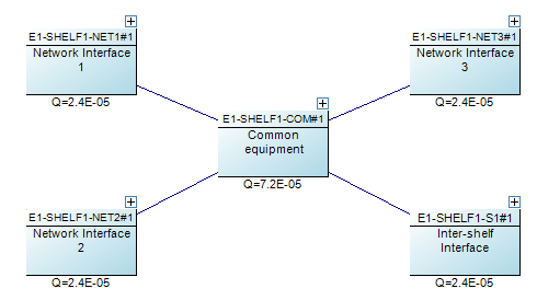
An example of a complex network element. The four network interfaces are each sockets, meaning any one of them could be used as an input or output to the network. The undirected connection means an availability path can be found going in either direction.
NAP also features a Parts library. Failure data is entered for these parts. In addition to standard failure rate or MTTF, which are quantities allowed in RBDs, NAP also has a Cable part type, which measures failures in cuts per distance per time. This makes it easier to model failures associated with the cable connection between two network elements. The Parts library also makes it easy to do "what if" analysis, by swapping similar components in and out of the block diagram, to evaluate how using a different BOM could impact the network availability.
NAP 2.0 represents the first update to the NAP software in several years. We've update the program to use the .NET framework, like our Reliability Workbench and Availability Workbench programs, which increases compatibility with modern Windows operating systems, and provides a more up-to-date user interface. It shares many new elements with our other applications, such as the Report Designer and Library facilities. Now, any NAP project can be opened as a library to facilitate sharing information between project files. Libraries also allow you to create common network elements and drag and drop them into your block diagram as needed.
NAP 2.0 is available exclusively as a 64-bit application.
Additionally, NAP 2.0 is in the first line of 64-bit applications we've ever released. You may have heard mention of 32-bit vs. 64-bit apps, or seen it in the context of Windows, e.g. Windows 7 32-bit version vs Windows 7 64-bit version, but not necessarily understood what exactly that means. It might sound a little bit like the computer nerd version of two car guys out-doing each other about the engine displacement of their muscle cars. "My '67 Camaro has a 283 cubic inch small block V8." "Oh, yeah? Well my '69 Challenger has a 426 Hemi!"
Basically, it refers to the amount of memory that can be accessed by the program or operating system. As an analogy, imagine a city planner designing a road and assigning addresses to the houses on the road. If he uses three-digit addresses for the houses, then the street could be a maximum of ten blocks long. However, if he uses four-digits, then he could have 100 blocks on a single street. Three digits may be all he needs for now, but if there are plans to further develop the neighborhood in the future, he might want to use four digits for the addresses.
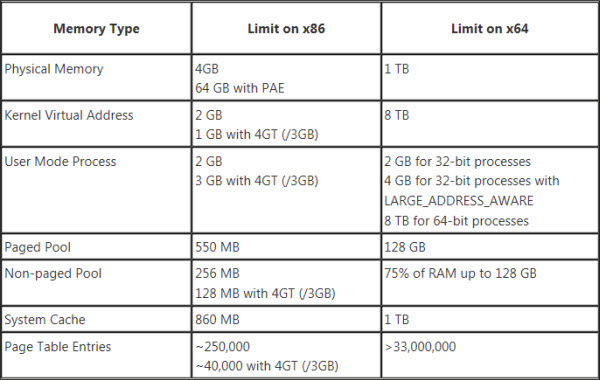
Computer memory works similarly: the number of bits for the operating system or the application refers to the number of blocks of memory that can be addressed and used. The maximum amount of memory you can address with 32 binary digits is about 4 gigabytes. Back in the mid-90s when the first 32-bit processors and applications were developed, that was an obscene amount of memory. However, the future has come and gone and now we can max out a computer with 32 gigabytes of memory for a little over $200. 32 bits is simply not enough to address all that memory, so about a decade ago, computer hardware and software began transitioning to 64 bit addressing. The maximum theoretical amount of memory you can address with 64 bits would be 16 exabytes (or about 16.8 million terabytes), although practical limitations with the hardware make it a lot lower. In other words, we don't have to worry about maxing that out anytime soon.
Honestly, I'm not sure I completely understand this either, but my Camaro has a 346 cu. in. small block V8!
Even if you were using a 64-bit version of Windows, a 32-bit app could only use a limited amount of memory. After the operating system takes its cut, the app is left with about two GB to work with. Most of the time, that's fine. If you're building a small- to medium-sized fault tree, that's more than enough. But NAP's undirected connections and sockets make path generation a complex affair, and the number of cut sets can increase exponentially with regard to the number of paths. More than any of our programs, NAP users were crashing into the limits of 32-bit computing, so this program will benefit most from the 64-bit version.
While the latest release of Reliability Workbench (12.1) comes in both 32- and 64-bit flavors, NAP 2.0 is only available as a 64-bit app. So knock yourself out and build the most complex network model you can think of. The only limitation is the hardware constraints of your computer!
NAP 2.0 is available as a free upgrade to users with a NAP license and current maintenance. Contact Isograph today to download or to renew your maintenance.
Thank you to everyone that attended our last meeting "building a Fault Tree from a schematic". I realize that there were many that were not able to attend the meeting. The warning that there are limited seats held true and the meeting did fill up leaving many of you to wonder what the proper logic was to modeling the schematic posted.
Not to worry, the meeting was recorded and can be accessed from the following link:
Since everyone in the meeting was muted watching the recording is almost as good as being there.
However, don't miss the chance to watch this weeks meeting live where we will be showing how to create various reports on the model we built last week. The same goes this week... please sign up to save a place in the meeting.
When modeling (or modelling for those of you in the UK) your system in a Fault Tree or Reliability Block Diagram do you ever wonder if your logic is covering all possible failures or properly accounting for redundancy in your system?
Try your hand at modelling the included schematic in a Fault Tree or Reliability Block Diagram (RBD) then join us on a Webniar, Friday at 10am PST, to see if your model matches up with the model one of our support experts comes up with. If you do not have access Fault Tree Analysis or RBD software please let me know and I will lend you software to use during this meeting.
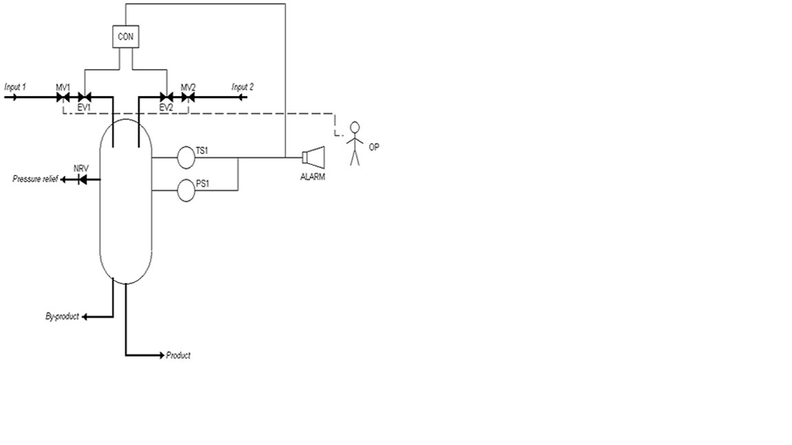
The safety system is designed to operate as follows: should a runaway reaction begin, the temperature sensor (TS1) and pressure sensor (PS1) will detect the increase in temperature and pressure and start the safe shutdown process. The provision of two sensors is for redundancy; only a single sensor needs to register the unsafe reactor conditions to engage the safety system. Should either TS1 or PS1 detect a runaway reaction, two things will occur: 1) a signal will be sent to the controller (CON), which will close the electric valves in each reactor input (EV1 and EV2), and 2) the alarm (ALARM) will sound, signaling the operator (OP) to close the manual valve in each reactor input (MV1 and MV2). In order to stop the runaway reaction, BOTH inputs must be shut down. However, only one valve on each input needs to be shut. So only MV1 or EV1 must be shut to stop input 1, but at least one valve on input 1 and at least one valve on input 2 must close to stop the inputs to the runaway reaction. Note that EV1 and EV2 (and only these components) are powered by the electrical grid; all other components have independent battery backups or power supplies.
Just in time for Thanksgiving we have announced our upcoming release of NAP 2. The development is in prototype stage so there is still opportunities to provide feedback prior to the final release. If you have any questions about NAP or would like to a closer look at some of the new features please let me know.
Howdy, folks! Isograph has recently launched Reliability Workbench 12, the latest incarnation of our flagship reliability analysis product. There are a number of new features and improvements, and today I'll be talking about a couple big changes.
The first and biggest change is the addition of a new Safety Assessment module. This new module allows users to perform Functional Hazard Analysis, PSSA analysis, and other safety assessments in accordance with SAE ARP 4761 and other similar standards.
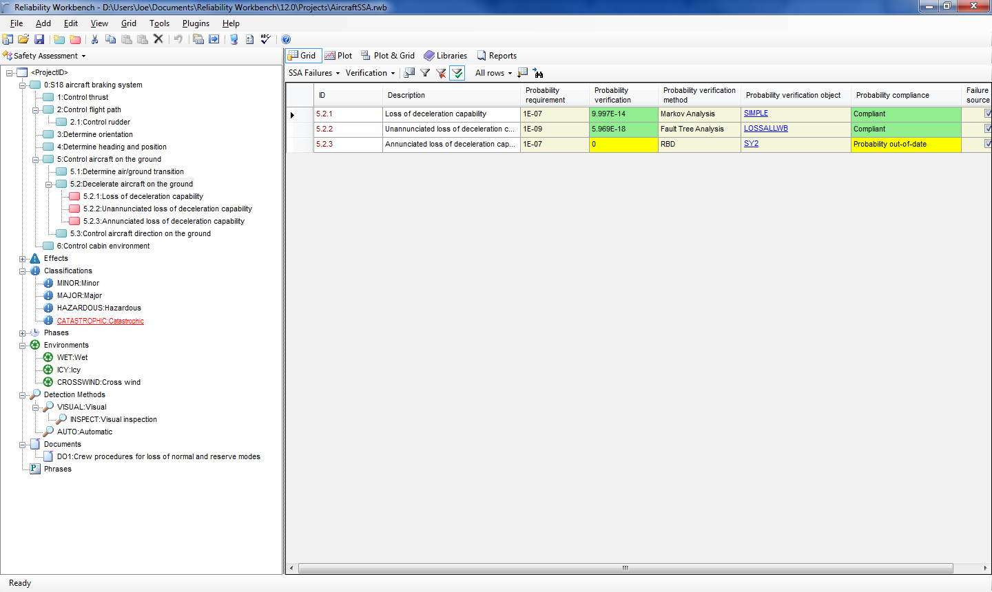
The System Safety Assessment (SSA) module allows users to construct a functional failure mode hierarchy, similar to the FMECA module of Reliability Workbench, or the RCMCost module of Availability Workbench. This functional hierarchy will list the functional requirements of the system, and the functional failures that could inhibit the system's ability to perform the functional requirements. So for instance, an aircraft braking system could have several functional requirements, such as control thrust, control aircraft on the ground, and decelerate aircraft on the ground. The "decelerate aircraft on the ground" function could fail if there is a loss of deceleration capability.
An example failure mode hierarchy.
Each failure can produce an effect. In our aircraft braking example, effects of failure of the braking system could be runway overrun, in which the aircraft is not able to completely decelerate the aircraft before the end of the runway. Then, each effect can have a user-defined classification, such as minor, major, or catastrophic. You can further define phases and conditions and tell the program that the effect only occurs during a particular phase or phases, and under specified conditions. For instance, the effect of a failure mode on an aircraft may only occur during take-off and landing, or in icy or wet conditions.
So far, so good. This isn't too different from what many users already use FMECA or RCMCost for. But what differentiates the SSA module is its ability to link to analyses in other modules, to provide justification that any safety or reliability targets have been met. Each effect classification in the SSA can have an assigned probability requirement associated with it. Then each failure mode can be linked to another analysis, either a Fault Tree, RBD, FMECA, Markov, or Prediction. The SSA module will then compare the probability requirement of the effect classification with the calculated probability from the other analysis to determine if the probability requirement is being met.
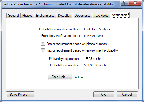
For example, in our aircraft overrun scenario, this effect is assigned a classification of catastrophic. The Powers That Be have decreed that catastrophic failure modes should not have a probability of greater than 1E-9 per hour. We can enter this information into the SSA module. Next, we can link the loss of deceleration capability failure mode to another analysis, perhaps a Fault Tree analysis, that calculates the probability of the failure mode's occurrence. The SSA module will then tell us if we're meeting our reliability target for the failure mode, based on the reliability analysis we've done.
While users have been building Fault Trees, RBDs, Markov models to verify a reliability target for years, the power of the System Safety Assessment module is that it can link all these analyses into a functional failure mode hierarchy. Previously, a user might have one Fault Tree to examine one critical system, then a Markov model to analyze another, with no organization or relation between the two. The power of the SSA module is that it allows users to combine all their reliability analyses into a single master project, showing all the failure modes of the system, and providing documented verification that reliability targets are being met. You can then print out reports showing the reliability targets and the reliability verified via quantitative analysis.
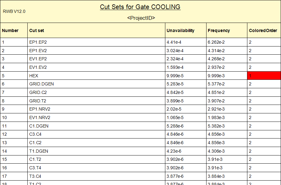
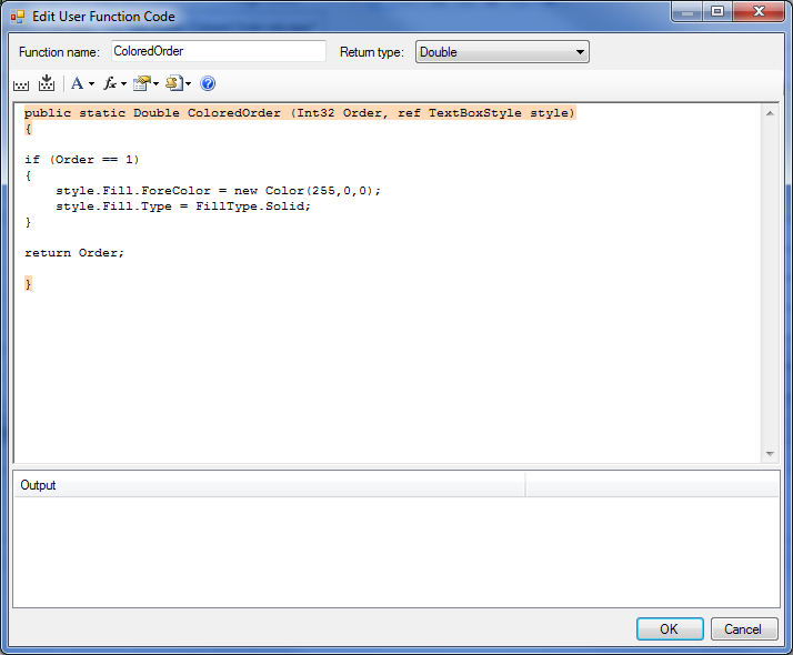
The other major new feature I want to talk about is User Columns in reports. User columns allow you to take the outputs from a report, then write simple code, either in Visual Basic or C# style, to create a new column in the report. Mostly, this is used to create conditional formatting, such that the font color, size, or style of a field in the report can be changed based on the value of that field, or of another field in the same row. But it can also be used to create more advanced columns, such as mathematical expressions, or logical conditions, that change the data displayed in a column. This could be used to change the units of a column, or combine multiple columns into one to, for instance, show either failure rate or characteristic life in a column, depending on whether the Rate or Weibull failure model is used.
An example of conditional formatting using User Columns that highlights first-order cut sets in red.The code used to generate the conditional formatting.
There are numerous other modifications and improvements that have been made in the latest release. You can read a summary of all the changes here. Customers with a current maintenance contract can upgrade for free, although you should contact us for a new license. Others can download a trial version to test it out. If you're interested in more information, or would like to upgrade, please give us a call or send us an email.
On August 4-8 Isograph sponsored the International Systems Safety Conference in St. Louis. This conference was the 32nd International System Safety Training Symposium. We enjoyed a great training symposium that focused on topics related to system safety discipline. Although any industry could benefit from this conference it seems to be engineers primarily from the aerospace industry attending this conference. Engineers take the time to exchange ideas, knowledge, experiences and best practices which gives the opportunity to learn from each other and share safety processes, methods, and techniques that advance the goals and objectives of the system safety profession. Isograph has now been supporting the Systems Safety Conference for almost 2 decades. To learn more about the Systems Safety Conference please go to their website: http://www.system-safety.org
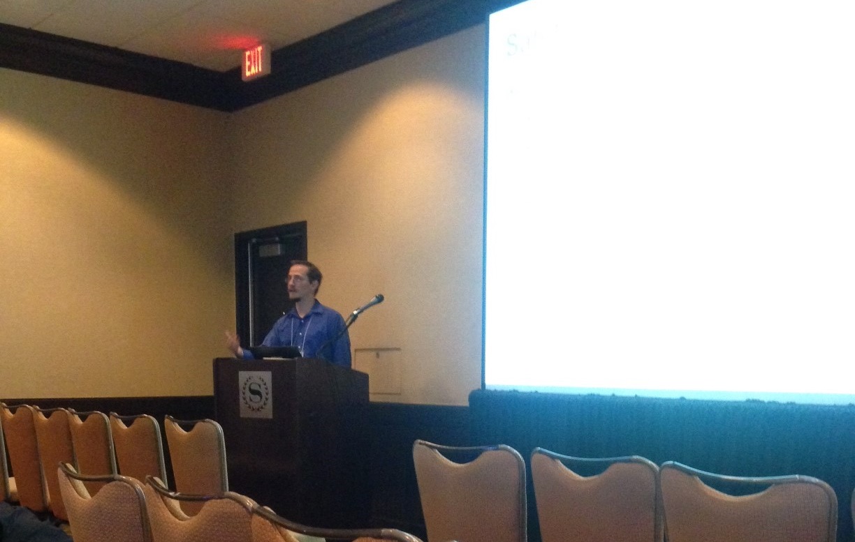
Howdy, folks. As Jeremy mentioned, we recently returned from Hawaii, where we were forced to go for the Probabilistic Safety Assessment & Management conference. We tried not to have too much fun in the sun between conference sessions. I also presented a paper, and I swear I had no idea where the conference was going to be when I submitted my abstract to the organizers. 😉 Anyways, the topic of my paper is great material for a Tech Tuesday post: Using Fault Trees to Analyze Safety-Instrumented Systems.
Yours truly, extolling the virtues of Fault Tree analysis
Safety-Instrumented Systems
Safety-Instrumented Systems (SIS) are designed to mitigate the risks of safety-critical processes or systems. Safety-critical systems are those that, if not properly maintained or controlled, can malfunction in such a way as to cause a significant risk to safety or another hazard. Examples of critical systems or processes are nuclear reactors, oil refineries, or even an automobile.
The SIS is designed to engage when the critical system experiences a failure. The SIS will automatically detect unsafe conditions in the critical system and prevent a hazard or restore the system to a safe state. An example of this might be an automated emergency shut-down in a reactor vessel, or even the airbag in a car. Due to their nature, SIS have stringent reliability requirements. When designing one, you need to know that it will work when required. This is where Fault Trees come into play. Using analytical FT methods, Reliability Workbench can evaluate the reliability of a SIS and help you determine its probability of failure on demand (PFD).
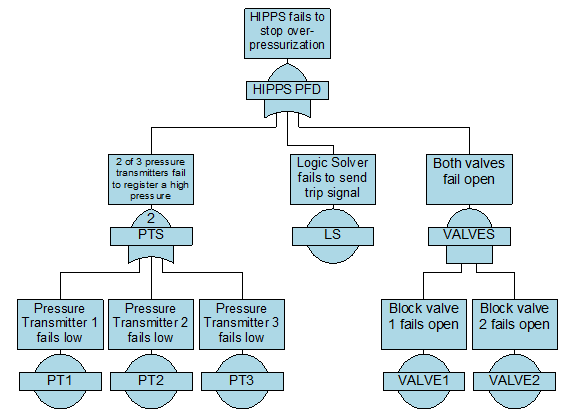
Take, for example, a high-integrity pressure protection system (HIPPS). This SIS is frequently see n in chemical plants and oil refineries. It is designed to prevent an over-pressurization event in a fluid line or vessel, by shutting off the input of the fluid.
High-Integrity Pressure Protection System
The example here consists of three pressure transmitters (PT), a logic solver, and two block valves. Two-out-of-three (2oo3) logic is applied to the pressure transmitters, meaning at least two of them must register the high pressure in order for the system to trip. Only one of the two block valves must close in order to stop the fluid flow. We can build a Fault Tree to represent this logic as such:
Failure Data
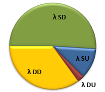
If you've read one of the standards that discusses safety-instrumented systems, such as IEC 61508, 61511, or ISO 26262, you may have seen this graph, representing the four failure modes of a typical component.
λ SD: Safe, Detected λ SU: Safe, Undetected λ DD: Dangerous, Detected, λ DU: Dangerous, Undetected
Safe failures are those that don't contribute to the PFD of the SIS, such as if the pressure transmitters in our HIPPS fail high. This failure won't inhibit the ability of the safety system to engage, since they are sending the signal to trip the SIS. Dangerous failures do contribute to PFD, like if the block valves fail open. Detected failures are those that are immediately known and can be corrected. Undetected failures remain hidden unless you test the component to see if it's still working. For Obvious Reasons, the dangerous, undetected failures are of the most concern.
In Reliability Workbench 11, Isograph added an IEC 61508 failure model to the program. This allows users to easily enter information for all four quadrants here; you can tell the program the overall failure rate, the dangerous failure percentage, and the diagnostic coverage for both safe and dangerous failures. The IEC 61508 failure model also allows for imperfect proof tests, so you can tell the program that some undetected failures remain undetected even after testing.
Common Cause Failures
One of the most important considerations when evaluating SIS are common cause failures (CCF). Standard probability math tells us that the probability of two random events occurring simultaneously is just the product of each individual events' probability. That is, to determine the probability that, say a coin flip lands heads and a die roll comes up 6, just multiply the probability of the coin landing heads by the probability of the die showing 6.
However, in SIS this is rarely the case due to common cause failures. CCFs basically mean that the random failures are not so random, and that components may be more likely to fail at the same time than you'd otherwise expect. For instance, the redundancy of the block valves means that you'd expect the probability of both of them to be failed to be the square of the individual probability of failure. However, due to CCFs, they are more likely to happen at the same time.
Reliability Workbench has a method of easily incorporating CCFs into the calculations. The most common method for taking these into account is called the beta factor model. With the beta factor CCF model, you can tell the program that a given percent of failures of a component are due to common causes, and all other components like it will also fail. For instance, we might say that the valves have a beta factor of 5%, meaning that 95% of their failures are random and independent, while the remaining 5% of failures of one will be due to causes that will also affect the other.
Logic Before Average
You may have heard that Fault Trees are unsuitable for solving SIS because of the way that the underlying Boolean algebra handles averaging probabilities. To an extent, what you've heard is correct. Typical Fault Tree methods can often provide optimistic results, predicting a PFD about 80% of the actual value. This is because Fault Tree methods first take an average PFD for each event, then apply the addition and multiplication laws of probability to solve for the system logic. However, SIS standards give equations that do the reverse. That is, they first apply logic, then solve for a PFD average. Since for a given function, the product of the means is not necessarily equal to the mean of the products, these two methods can produce different results.
To account for this, Reliability Workbench provides a special "logic before average" calculation method, which brings its results in line with the answers calculated using IEC 61508 methods. These proprietary calculations were first included in FaultTree+ v11, released in 2005.
Spurious Trips
Spurious trips are failures of the safety system, but in a "safe" way. That is, they are false alarms, where the SIS engages when no hazardous condition was present, due to safe failures of the components. For instance, if two of the pressure transmitters in our HIPPS were to fail high, this would send a signal to engage the SIS, even though there was no actual high pressure. While spurious trips often don't carry the same hazardous consequences that a dangerous failure does, the can be annoying and costly, because they probably involve stopping a process, which may take several hours to restart, leading to loss of production.
In some serious cases, spurious trips are more safety-critical than demand failures. Consider, for instance, the airbag on your car. If it fails to go off when needed, there's a greater chance that you'll be injured than if it had deployed. However, if it deploys when not needed, say when you're driving along at 70 mph on the highway, then it can cause you to lose control of the car and cause an accident.
One very useful feature about using Reliability Workbench to analyze SIS is the inclusion of features to easily perform spurious trip analysis. If your using the IEC 61508 failure model, then you've already entered information pertaining to safe failure rate. If you just apply some logical reversals—and again, there's a feature to automatically do this for you—then the Fault Tree can very easily be reconfigured to solve for the mean time to fail spuriously (MTTFspurious).
PFDavg
λ (/hour)
MTBF (hours)
RRF
Spurious trip rate (/hour)
MTTFspurious (hours)
4.7E-3
6.193E-7
1,622,000
212.8
6.165E-6
162,200
HIPPS final analysis
There was one more section to my PSAM 12 paper, but I've already discussed it here: importance and sensitivity analysis. If you're interested in leaning more about this, Isograph offers a two-day SIS in Fault Tree training course, which covers Fault Tree basics and shows how to model complex SIS logic in the Reliability Workbench.
So there you have it; while our wives were stuck outside, basking in the sun and drinking tropical beverages from coconut shells, Jeremy and I were having a grand time at the conference, talking about how great Fault Trees are for analyzing SIS. I'm sure our wives were so jealous that they weren't able to attend the presentation.
My wife contemplates what she's missing out on by not being at the conference.
This years PSAM took place on the beautiful island of Oahu, Hawaii. Begrudgingly we packed our bags last week and headed to Hawaii. Although I might have been hoping for some sun and surf the conference was all business. The Probabilistic Safety Assessment & Management conference is a conference in risk, risk management, reliability, safety, and associated topics. Historically this conference has been attended primarily by the nuclear industry. This years PSAM was a mixture of several different industries, the nuclear industry making up about half the attendees.
The PSAM conference brings together experts from various industries. The multi-disciplinary conference is aimed to cross-fertilize methods, technologies and ideas for the benefit of all. PSAM meets internationally every two years. This years conference was in Hawaii, 2016 will be in Korea. http://psam12.org
This week Isograph attended the CIM (Canadian Institute of Mining) conference in Vancouver, http://vancouver2014.cim.org/ which was a great event. As software authors we usually don't get the chance to take a close look at the machinery that is often modeled in our software. The CIM conference not only gave us this chance it seemed to have a bit of everything including: 12 foot tires, 14 ton trucks, UAV's, drills, software and many items specific to the mining industry. Its also the only conference I have been to that had its own fireworks show!
CIM is a very mature organization which was founded in 1898, the Canadian Institute of Mining, Metallurgy and Petroleum (CIM) is the leading technical society of professionals in the Canadian Minerals, Metals, Materials and Energy Industries. CIM has over 14,600 members, convened from industry, academia and government. With 10 Technical Societies and over 35 Branches, their members help shape, lead and connect Canada’s mining industry, both within Canadian borders and across the globe. Canadian Institute of Mining - 2014
Let's Keep In Touch!
Subscribe to our newsletter to get the latest information on Isograph software.